Constrained Tikhonov regularization implemented by (accelerated) forward-backward splitting

We consider the two-dimensional deconvolution problems to find a non-negative function f given data

\[d \sim \mathrm{Pois}(h*f)\]

with a non-negative convolution kernel \(h\), and \(\mathrm{Pois}\) denotes the element-wise Poisson distribution.

We explore the use of the semismooth Newton method to implement constrained Tikhonov regularization

\[\hat{f} = \mathrm{argmin}_{f\geq 0} \left[\| h*f-d\|^2_{L^2(w)} + \alpha \|f\|^2_{L^2}\right]\]

with a weight \(w = \frac{1}{\sqrt{d+1}}\). The regularization parameter \(\alpha\) is chosen such that the duality gap is small.

import numpy as np
from regpy.operators.convolution import GaussianBlur
from regpy.vecsps import UniformGridFcts
from regpy.solvers import TikhonovRegularizationSetting
from regpy.solvers.linear.proximal_gradient import ForwardBackwardSplitting, FISTA
from regpy.hilbert import L2, HmDomain
from regpy.stoprules import CountIterations, DualityGapStopping

Logging

For the logging of each subroutine we will rely on the loglevel INFO to obtain certain information and predefine a format for the logging.

import logging

logging.basicConfig(
    level=logging.INFO,
    format='%(asctime)s %(levelname)s %(name)-20s :: %(message)s'
)

Plotting routine

To be able to later plot easily and consistently we define a routine to plot the images using matplotlib.pyplot

import matplotlib.pyplot as plt
import matplotlib as mplib

def comparison_plot(grid,truth,reco,title_right='exact',title_left='reconstruction',residual=None):
    plt.rcParams.update({'font.size': 22})
    extent = [grid.axes[0][0],grid.axes[0][-1], grid.axes[1][0], grid.axes[1][-1]]
    maxval = np.max(truth[:]); minval = np.min(truth[:])
    mycmap = mplib.colormaps['hot']
    mycmap.set_over((0,0,1.,1.))  # use blue as access color for large values
    mycmap.set_under((0,1,0,1.))  # use green as access color for small values
    if not (residual is None):
        fig, ((ax1,ax2),(ax3,ax4)) = plt.subplots(2,2,figsize = (22,16))
    else:
        fig, (ax1,ax2) = plt.subplots(1,2,figsize = (22,8))
    im1= ax1.imshow(reco.T,extent=extent,origin='lower',
                    vmin=1.05*minval-0.05*maxval, vmax =1.05*maxval-0.05*minval,
                    cmap=mycmap
                    )
    ax1.title.set_text(title_left)
    fig.colorbar(im1,extend='both')
    im2= ax2.imshow(truth.T,extent=extent, origin='lower',
                    vmin=1.05*minval-0.05*maxval, vmax =1.05*maxval-0.05*minval,
                    cmap=mycmap
                    )
    ax2.title.set_text(title_right)
    fig.colorbar(im2,extend='both',orientation='vertical')
    if not (residual is None):
        maxv = np.max(reco[:]-truth[:])
        im3 = ax3.imshow(truth.T-reco.T,extent=extent, origin='lower',vmin= -maxv,vmax=maxv,cmap='RdYlBu_r')
        ax3.title.set_text('reconstruction error')
        fig.colorbar(im3)

        maxv = np.max(residual[:])
        im4 = ax4.imshow(residual.T,extent=extent, origin='lower',vmin= -maxv,vmax=maxv,cmap='RdYlBu_r')
        ax4.title.set_text('data residual')
        fig.colorbar(im4)

2025-08-13 09:02:51,100 INFO matplotlib.font_manager :: generated new fontManager

Test object

The exact solution is constructed by a ring a box and an cross above and some decreasing bubbles on the bottom.

grid = UniformGridFcts((-1, 1, 256), (-1.5, 1, 256),dtype = float, periodic = True)
"""Space of real-valued functions on a uniform grid with rectangular pixels"""
X = grid.coords[0]; Y = grid.coords[1]
"""x and y coordinates."""
cross = 1.0*np.logical_or((abs(X)<0.01) * (abs(Y)<0.3),(abs(X)<0.3) * (abs(Y)<0.01))
rad = np.sqrt(X**2 + Y**2)
ring = 1.0*np.logical_and(rad>=0.9, rad<=0.95)
smallbox = (abs(X+0.55)<=0.05) * (abs(Y-0.55)<=0.05)
bubbles = (1.001+np.sin(50/(X+1.3)))*np.exp(-((Y+1.25)/0.1)**2)*(X>-0.8)*(X<0.8)

ramp = Y<=-1

objects = 200*(ring + 2.0*cross + 1.5*smallbox + 2*ramp -bubbles)
exact_sol = objects

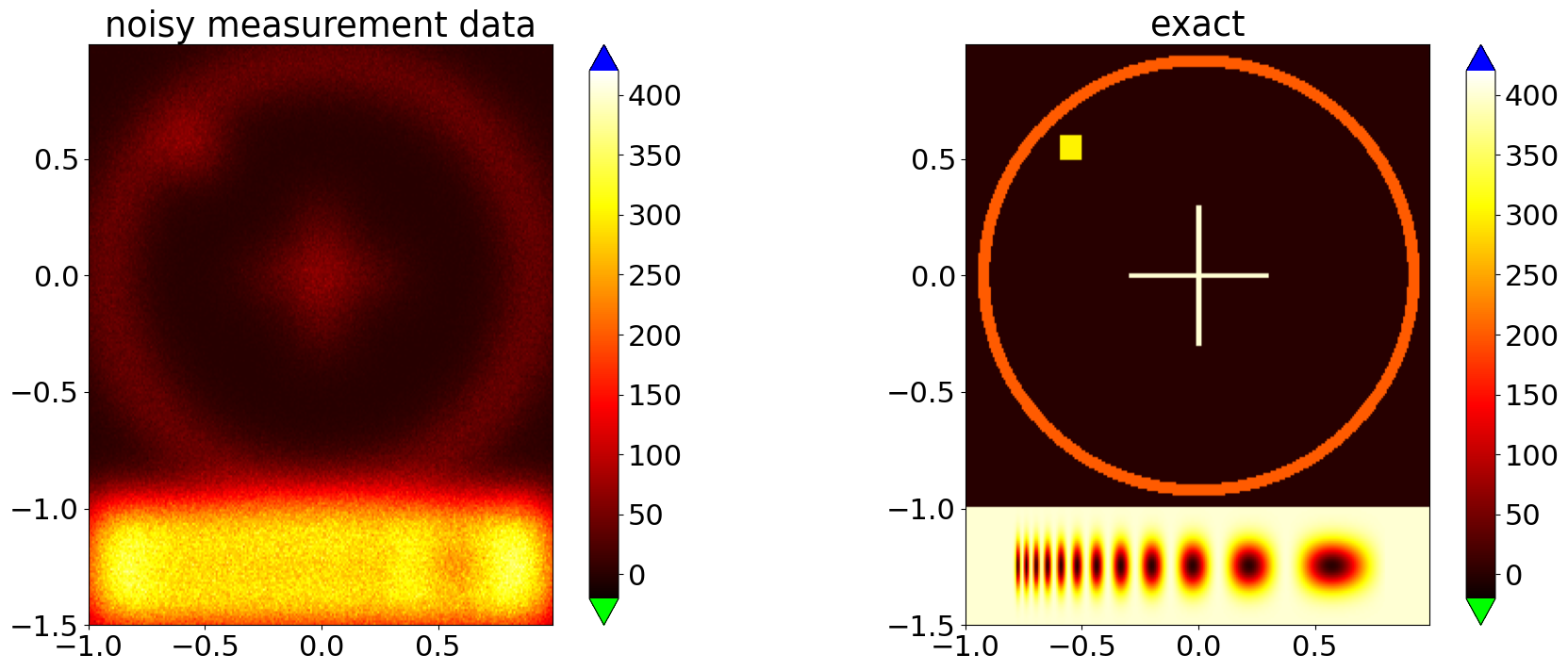
creating synthetic data

Using the np.random.poisson we construct poisson data from a Gaussian blur of the true solution. The Gaussian blur is constructed with the GaussianBlur convolution operator of RegPy.

a=0.15
conv =  GaussianBlur(grid,a,pad_amount=((16,16),(16,16)))
"""Convolution operator \(f\mapsto h*f\) for the convolution kernel \(h(x)=\exp(-|x|_2^2/a^2)\)."""
blur = conv(exact_sol)
blur[blur<0] = 0.
"""Simulated exact data."""
data = np.random.poisson(blur)
"""Simulated measured data. The Poisson distribution occurs if photon count detectors are used."""
comparison_plot(grid,exact_sol,data,title_left='noisy measurement data')

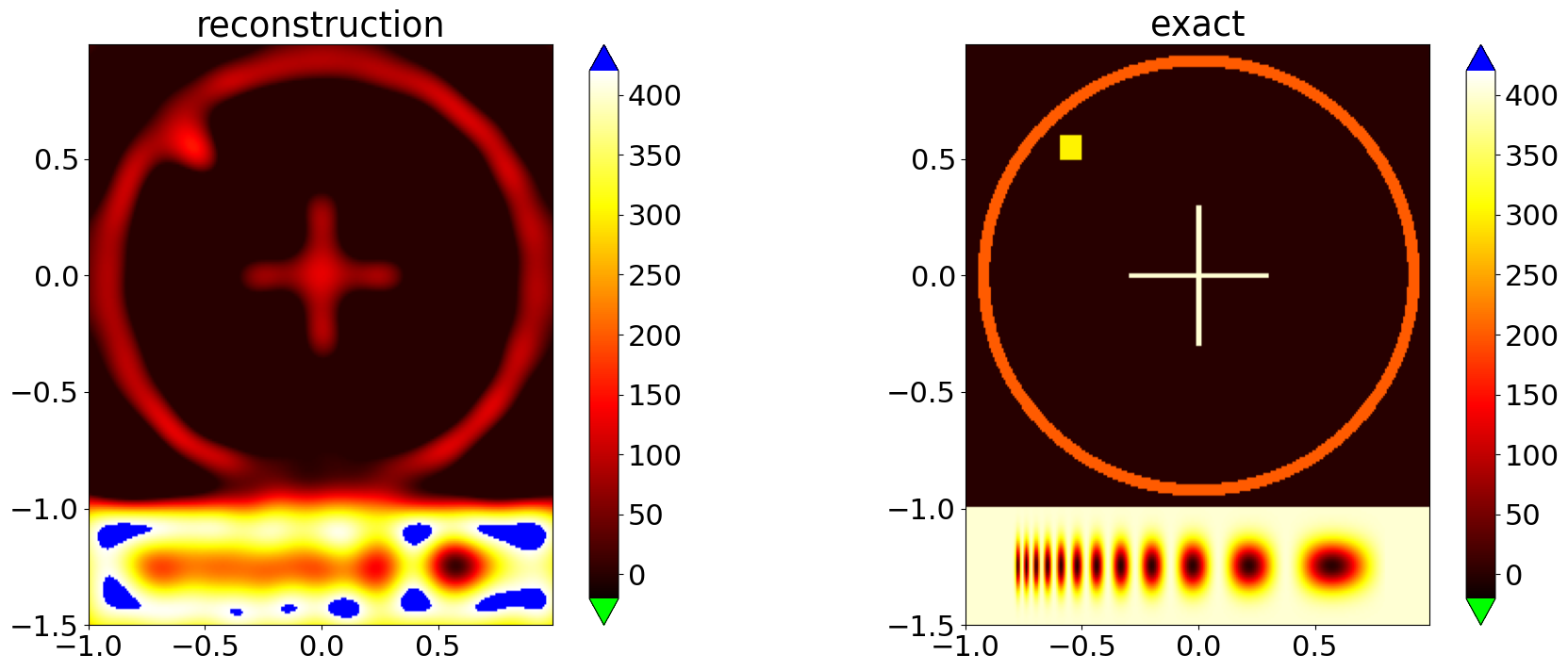
Reconstruction by Forward-Backward Splitting

We split the Tikhonov functional into the quadratic data fidelity term and a penalty term, which also includes the nonnegativity constraint. Then we setup a solver using the forward-backward splitting and FISTA to solve the Tikhonov functional.

Note that we allow in the quadratic bilateral constraint small violations of the bounds to prevent the evaluation to be infinite.

from regpy.functionals import QuadraticBilateralConstraints

weighted_data_space = L2(grid, weights = 1./(1.+data))
pen = QuadraticBilateralConstraints(grid,lb=0,ub=400*conv.domain.ones(),x0=0,eps=0.0001)
alpha = 0.001
setting = TikhonovRegularizationSetting(op=conv, penalty=pen, data_fid = weighted_data_space,data_fid_shift=data,regpar=alpha)

solver_FB = ForwardBackwardSplitting(setting)
solver_FISTA = FISTA(setting)

2025-08-13 09:02:53,946 INFO FISTA                :: Setting up FISTA with convexity parameters mu_R=1.000e-03, mu_S=0.000e+00 and step length tau=2.198e+00.
 Expected linear convergence rate: 9.532e-01

Solving the inverse problem

Using a stopping rule defined using the measure of the duality gap we solve run the solver.

from regpy.stoprules import DualityGapStopping

stoprule=DualityGapStopping(solver_FB,threshold = 1., max_iter=1500,logging_level=logging.WARNING)
x,y = solver_FB.run(stoprule)
comparison_plot(grid,exact_sol,x)
stoprule=DualityGapStopping(solver_FISTA,threshold = 1., max_iter=150,logging_level=logging.WARNING)
x,y = solver_FISTA.run(stoprule)
comparison_plot(grid,exact_sol,x)

2025-08-13 09:03:02,591 INFO ForwardBackwardSplitting :: Solver converged after 1148 iteration.
2025-08-13 09:03:03,437 INFO FISTA                :: Solver converged after 121 iteration.

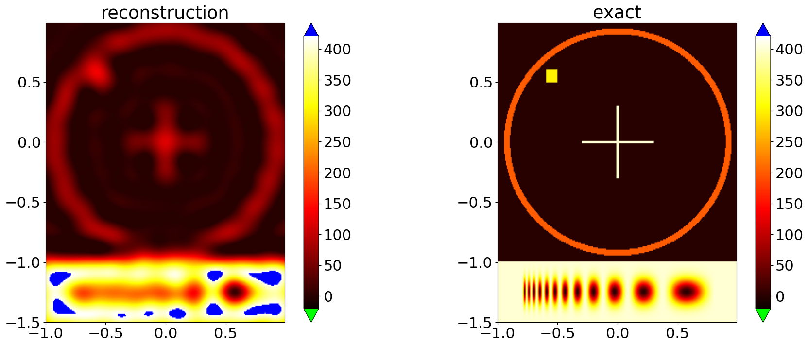
Reconstruction with one sided constraints

Other than using a bilateral constraint we may only use a lower bound quadratic constraint. Then we have to redefine the setting and define new solvers and then invert.

from regpy.functionals import QuadraticLowerBound
weighted_data_space = L2(grid, weights = 1./(1.+data))
alpha = 1e-3
pen = QuadraticLowerBound(grid,grid.zeros(), 50*grid.ones())
setting = TikhonovRegularizationSetting(op=conv, penalty=pen, data_fid = L2,data_fid_shift=data,regpar=alpha)
solver_FB = ForwardBackwardSplitting(setting,grid.zeros())
solver_FISTA = FISTA(setting)

stoprule=DualityGapStopping(solver_FB,threshold = 1., max_iter=2500,logging_level=logging.WARNING)
x,y = solver_FB.run(stoprule)
comparison_plot(grid,exact_sol,x)
stoprule=DualityGapStopping(solver_FISTA,threshold = 1., max_iter=200,logging_level=logging.WARNING)
x,y = solver_FISTA.run(stoprule)
comparison_plot(grid,exact_sol,x)

2025-08-13 09:03:06,758 INFO FISTA                :: Setting up FISTA with convexity parameters mu_R=1.000e-03, mu_S=0.000e+00 and step length tau=1.042e+00.
 Expected linear convergence rate: 9.677e-01
2025-08-13 09:03:19,629 INFO ForwardBackwardSplitting :: Solver converged after 1919 iteration.
2025-08-13 09:03:20,943 INFO FISTA                :: Solver converged after 175 iteration.

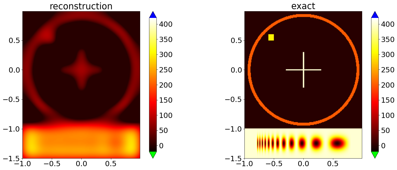
Reconstruction without constraints

To compare to the previous reconstructions we use a standard \(L^2\) penalty and only after the reconstruction we use a cut to compare the results.

weighted_data_space = L2(grid, weights = 1./(1.+data))
alpha = 1e-3
pen = L2
setting = TikhonovRegularizationSetting(op=conv, penalty=pen, data_fid = L2,data_fid_shift=data,regpar=alpha)
setting.penalty
solver_FB = ForwardBackwardSplitting(setting,grid.zeros())
solver_FISTA = FISTA(setting)

stoprule=DualityGapStopping(solver_FB,threshold = 1., max_iter=2500,logging_level=logging.WARNING)
x,y = solver_FB.run(stoprule)
x=np.maximum(x,0)
comparison_plot(grid,exact_sol,x)
stoprule=DualityGapStopping(solver_FISTA,threshold = 1., max_iter=200,logging_level=logging.WARNING)
x,y = solver_FISTA.run(stoprule)
x=np.maximum(x,0)
comparison_plot(grid,exact_sol,x)

2025-08-13 09:03:23,942 INFO FISTA                :: Setting up FISTA with convexity parameters mu_R=1.000e-03, mu_S=0.000e+00 and step length tau=1.042e+00.
 Expected linear convergence rate: 9.677e-01
2025-08-13 09:03:35,615 INFO ForwardBackwardSplitting :: Solver converged after 1784 iteration.
2025-08-13 09:03:36,915 INFO FISTA                :: Solver converged after 200 iteration.