Parallel Magnetic Resonance imaging (MRI)

Standard MRI is described by the Fourier transform \(\mathcal{F}\) as forward operator (here in two dimensions). To accelerate data acquisition, parallel MRI uses simultaneous measurements by \(N\) receiver coils. This allows undersampling of the Fourier domain leading to speed-ups. Parallel MRI is described by the forward operator

\[\begin{split}F\left(\begin{array}{c}\rho \\ c_1\\ \vdots \\ c_N\end{array}\right) = \left(\begin{array}{c}M\cdot\mathcal{F}(c_1 \cdot \rho)\\ \vdots \\ M\cdot\mathcal{F}(c_N \cdot \rho)\end{array}\right).\end{split}\]

Here \(\rho\) describes the hydrogen density and is the main quantity of interest. To take into account effects such as motion artifacts, \(\rho\) has to be modeled as a complex-valued function. \(c_1,\dots, c_N\) describe complex-valued coil profile, which may be assumed to be smooth. As they depend on the sample \(\rho\), they must be reconstructed together with \(\rho\). \(M\) is a 0-1-mask describing the undersampling pattern.

import matplotlib.pyplot as plt
import matplotlib as mplib
from matplotlib.colors import hsv_to_rgb
import numpy as np
from scipy.io import loadmat

Defining the operators

We define a general coil-multiplication operator that multiplies the complex coil profiles by the hydrogen density. Composing it with a Fourier transform in the non-stacked directions yields the parallel-MRI operator.

from regpy.vecsps import UniformGridFcts
from regpy.operators import Operator, FourierTransform, DirectSum, PtwMultiplication

class CoilMult(Operator):
    """Operator that implements the multiplication between density and coil profiles. The domain
    is a direct sum of the `grid` (for the densitiy) and a `regpy.vecsps.UniformGridFcts` of `ncoils`
    copies of `grid`, stacked along the 0th dimension.

    Parameters
    ----------
    grid : regpy.vecsps.UniformGridFcts
        The grid on which the density is defined.
    ncoils : int
        The number of coils.
    """

    def __init__(self, grid, ncoils):
        assert isinstance(grid, UniformGridFcts)
        assert grid.ndim == 2
        self.grid = grid
        """The density grid."""
        if(ncoils>1):
            self.coilgrid = UniformGridFcts(ncoils, *grid.axes, dtype=grid.dtype)
        else:
            self.coilgrid=UniformGridFcts(*grid.axes, dtype=grid.dtype)
        """The coil grid, a stack of copies of `grid`."""
        self.ncoils = ncoils
        """The number of coils."""
        super().__init__(
            domain=self.grid + self.coilgrid,
            codomain=self.coilgrid
        )

    def _eval(self, x, differentiate=False, adjoint_derivative=False):
        density, coils = self.domain.split(x)
        if differentiate or adjoint_derivative:
            r"""We need to copy here since `.split()` returns views into `x` if possible."""
            self._density = density.copy()
            self._coils = coils.copy()
        return density * coils

    def _derivative(self, x):
        density, coils = self.domain.split(x)
        return density * self._coils + self._density * coils

    def _adjoint(self, y):
        density = self._density
        coils = self._coils
        if self.grid.is_complex:
            r"""Only `conj()` in complex case. For real case, we can avoid the copy."""
            density = np.conj(density)
            coils = np.conj(coils)
        if(self.ncoils>1):
            return self.domain.join(
                np.sum(coils * y, axis=0),
                density * y)
        return self.domain.join(coils*y,density*y)

def parallel_mri(grid, ncoils, centered=False):
    """Construct a parallel MRI operator by composing a `regpy.operators.FourierTransform` and a
    `CoilMult`. Subsampling patterns need to added by composing with e.g. a `cartesian_sampling`.

    Parameters
    ----------
    grid : vecsps.UniformGridFcts
        The grid on which the density is defined.
    ncoils : int
        The number of coils.
    centered : bool
        Whether to use a centered FFT. If true, the operator will use fftshift.

    Returns
    -------
    Operator
    """
    cmult = CoilMult(grid, ncoils)
    ft = FourierTransform(cmult.codomain, axes=range(1, cmult.codomain.ndim), centered=centered)
    return ft * cmult

Partial Sobolev initialization

Partial reimplementation of the Sobolev Gram matrix. Can be composed with forward operator (from the right) to substitute coils = ifft(aux / sqrt(sobolev_weights)), making aux the new unknown. This can be used to avoid the numerically unstable Gram matrix for high Sobolev indices.

def sobolev_smoother(codomain, sobolev_index, factor=None, centered=False):
    """
    Parameters
    ----------
    codomain :
        Codomain of the operator
    sobolev_index : int
    centered : bool
        Whether to use a centered FFT. If true, the operator will use fftshift.
    factor : float
        If factor is None (default): Implicit scaling based on the codomain. Otherwise,
        the coordinates are normalized and this factor is applied.
    """
    grid, coilsgrid = codomain
    ft = FourierTransform(coilsgrid, axes=(1, 2), centered=centered)
    ft_codomain_coord_slice=np.asarray(ft.codomain.coords[1:])
    if factor is None:
       mulfactor = grid.volume_elem * (
                    1 + np.linalg.norm(ft_codomain_coord_slice, axis=0)**2
                                      )**(-sobolev_index / 2)
    else:
        mulfactor = ( 1 + factor * np.linalg.norm(ft_codomain_coord_slice/2./np.amax(np.abs(ft_codomain_coord_slice)), axis=0)**2
                                                 )**(-sobolev_index / 2)

    mul = PtwMultiplication(ft.codomain, mulfactor)
    return DirectSum(grid.identity, ft.inverse * mul, codomain=codomain)

Estimating the sampling pattern

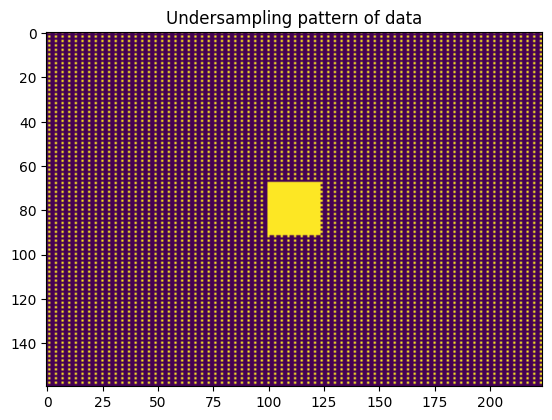
Estimate the sampling pattern from measured data is very important. Here we have a short method, that if some measurement point is zero in all coil profiles it is assumed to be outside of the sampling pattern. This method has a very low probability of failing, especially non-integer data.

def estimate_sampling_pattern(data):
    return np.all(data != 0, axis=0)

Complex to rgb conversion

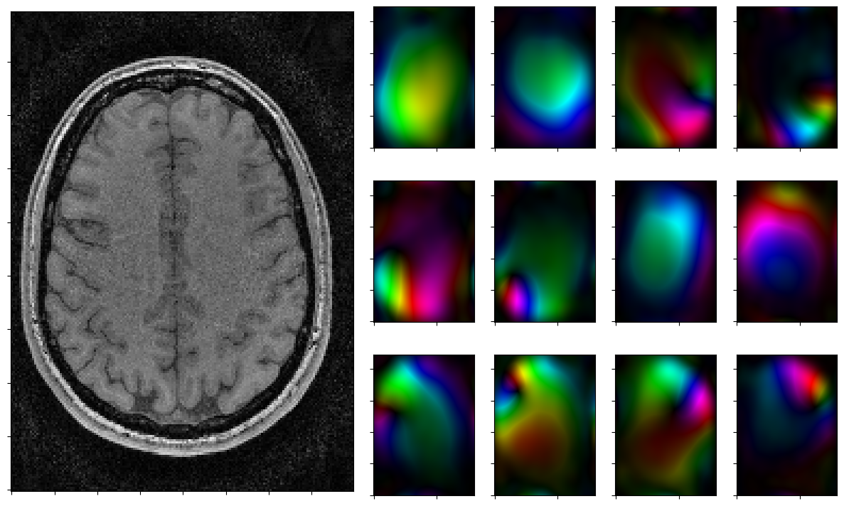
To plot the complex coil profiles we need to convert the complex arrays to rgb. The following method converts array of complex numbers into array of RGB color values for plotting. The hue corresponds to the argument. The brightness corresponds to the absolute value.

Parameters >z : numpy.ndarray >array of complex numbers

Returns > numpy.ndarray > Array that contains three values for each value in z containing the RGB representation of this value.

def complex_to_rgb(z):
    HSV = np.dstack( (np.mod(np.angle(z)/(2.*np.pi),1), 1.0*np.ones(z.shape), np.abs(z)/np.max((np.abs(z[:]))), ))
    return hsv_to_rgb(HSV)

Load data from file and estimate sampling pattern

Here we load the data from a stored file normalize it and extract the number of coils, and shape. Using this information we can define the space for each coil profile as a uniform grid of complex valued functions. Finally, we use the data to extract the mask of the sampling pattern and we plot that sampling pattern.

data = loadmat('../../../../examples/mri/data/ksp3x2.mat')['Y']
data = np.transpose(data,(2,0,1))*(100/np.linalg.norm(data))
# normalize and transpose data
nrcoils,n1,n2 = data.shape
grid = UniformGridFcts((-1, 1, n1), (-1, 1, n2), dtype=complex)
mask = estimate_sampling_pattern(data)
plt.imshow(mask.T); plt.title('Undersampling pattern of data')

Text(0.5, 1.0, 'Undersampling pattern of data')

Set up forward operator

With the coil grid and number of coils defined, we can construct the MRI operator. We first create the full operator without a sampling pattern. We then apply the sampling mask by pointwise multiplication and add the Sobolev smoother. Incorporating the smoothing into the operator avoids adding it later in the setting and solver. Composing these components yields the final parallel-MRI operator.

sobolev_index = 32

full_mri_op = parallel_mri(grid=grid, ncoils=nrcoils,centered=True)
sampling = PtwMultiplication(full_mri_op.codomain,(1.+0j)* mask)
smoother = sobolev_smoother(full_mri_op.domain, sobolev_index, factor=220.)

parallel_mri_op = sampling * full_mri_op * smoother

Set up initial guess

As an initial guess we use constant density and zero coil profiles. First we split the composed zero vector and then we set the density to constant one. Note we use init_density[...] = 1 to have a mutable operation on the variable.

init = parallel_mri_op.domain.zeros()
init_density, _ = parallel_mri_op.domain.split(init)
init_density[...] = 1

Set up regularization method

With the operator, data, and initial guess defined, we can construct the setting, solver, and stopping rule. The iteratively regularized Gauss–Newton method is stopped after five iterations.

from regpy.stoprules import CountIterations
from regpy.solvers import Setting
from regpy.solvers.nonlinear.irgnm import IrgnmCG
from regpy.hilbert import L2

setting = Setting(op=parallel_mri_op, penalty=L2, data_fid=L2, data = data, regpar=1.)

solver = IrgnmCG(
    setting=setting,
    regpar_step=1/3.,
    init=init
)

stoprule = CountIterations(max_iterations=5)

Run solver by hand and plot iterates

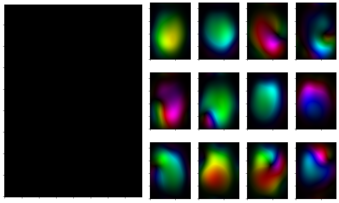
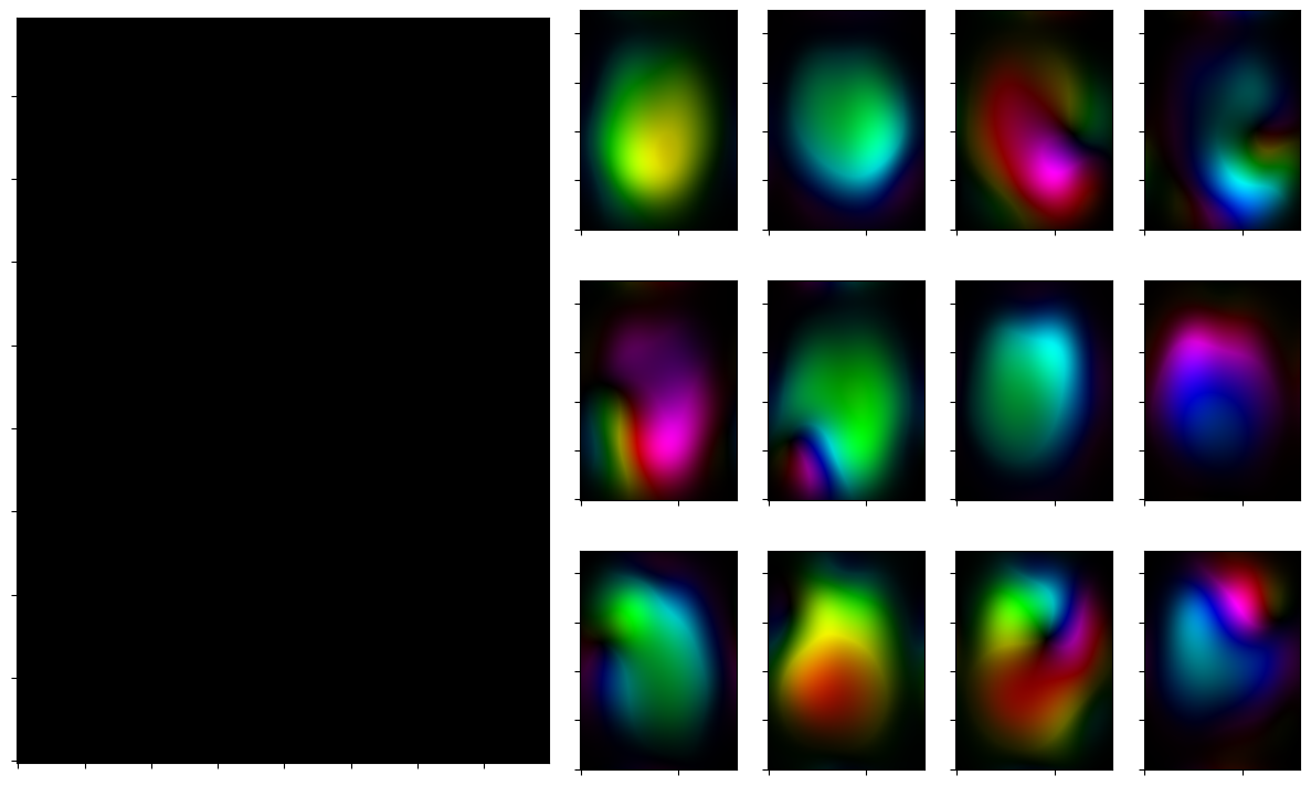
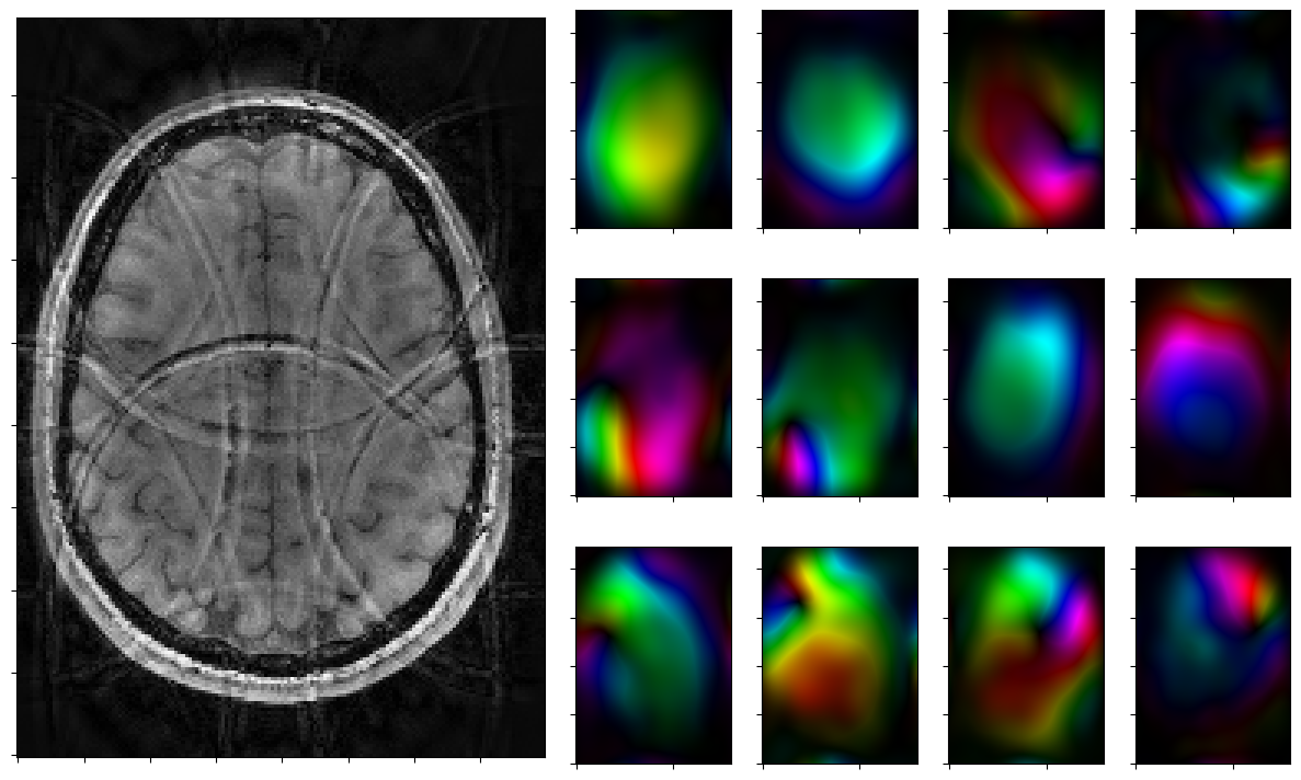
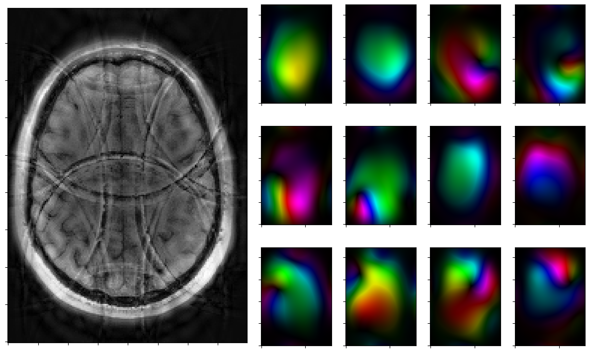
Run the solver iteratively and plot each step.

for reco, reco_data in solver.while_(stoprule):
    rho, coils = smoother.codomain.split(smoother(reco))
    #rho, coils = normalize(rho,coils)

    fig = plt.figure(figsize = (15,9))

    gs = fig.add_gridspec(3,7)
    axs = [fig.add_subplot(gs[0:3, 0:3])]
    axs[0].imshow(np.abs(rho),cmap=mplib.colormaps['Greys_r'],origin='lower')
    axs[0].xaxis.set_ticklabels([])
    axs[0].yaxis.set_ticklabels([])
    for j in range(3):
        for k in range(3,7):
            axs.append(fig.add_subplot(gs[j,k]))
            axs[-1].xaxis.set_ticklabels([])
            axs[-1].yaxis.set_ticklabels([])
    for j in range(nrcoils):
        axs[1+j].imshow(complex_to_rgb(coils[j,:,:]),origin='lower')
    plt.show()