[1]:
import numpy as np
import matplotlib.pyplot as plt

from regpy.operators import Operator
from regpy.vecsps import UniformGridFcts
Volterra example with iterative regularised Gauss-Newton semismooth solver
The discrete Volterra operator. The Volterra operator \(V_n\) is defined as
Its discrete form, using a Riemann sum, is simply
where \(h\) is the grid spacing. \(V_1\) is linear.
Therefore, we create a subclass of regpy.Operator type in the next code block. In the following create new operators of that type can simply be done by initiating with that class. This class will have the following parameters. (Side remark you may also do the definition in a separate file for this example check out volterra.py in this example folder. )
Parameters
domain : regpy.vecsps.UniformGridFcts > The domain on which the operator is defined. Must be one-dimensional.
exponent : float > The exponent (n). Default is 1.
[2]:
class Volterra(Operator):
    def __init__(self, domain, exponent=1):
        assert isinstance(domain, UniformGridFcts)
        assert domain.ndim == 1
        self.exponent = exponent
        """The exponent."""
        super().__init__(domain, domain, linear=(exponent == 1))

    def _eval(self, x, differentiate=False):
        if differentiate:
            self._factor = self.exponent * x**(self.exponent - 1)
        return self.domain.volume_elem * np.cumsum(x**self.exponent)

    def _derivative(self, x):
        return self.domain.volume_elem * np.cumsum(self._factor * x)

    def _adjoint(self, y):
        x = self.domain.volume_elem * np.flipud(np.cumsum(np.flipud(y)))
        if self.linear:
            return x
        else:
            return self._factor * x
Initialization
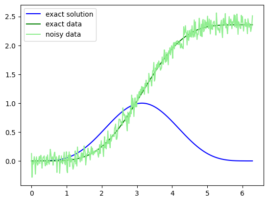
Having generally defined the Volterra operator above construct an explicit Volterra operator with exponent \(n=2\) on the interval \([0,2\pi]\) discretized by a UniformGridFcts with 200 points. Note, the operator will be non-linear operator since the exponent is not \(1\). Moreover, we choose the exact solution
for which the exact data is given by
Additionally we construct noise by sampling in the codomain a random vector. This noise \(\nu\) is then added to the exact data giving our noisy data \(g^\delta = g^\dagger + \nu\).
[3]:
grid = UniformGridFcts(np.linspace(0, 2 * np.pi, 400))
op = Volterra(grid,exponent=2)

exact_solution = (1-np.cos(grid.coords[0]))**2/4
plt.figure()
plt.plot(grid.coords[0],exact_solution,color="blue",label='exact solution')

exact_data = (3*grid.coords[0] - 4*np.sin(grid.coords[0]) + np.cos(grid.coords[0])*np.sin(grid.coords[0]))/8
noise = 0.1 * op.codomain.randn()
data = exact_data + noise
plt.plot(grid.coords[0], exact_data, color="green", label='exact data')
plt.plot(grid.coords[0], data, color="lightgreen", label='noisy data')
plt.legend()

print("Maximal error of operator evaluation on exact solution to exact data: {:.4E}".format(np.max(np.abs(op(exact_solution)-exact_data))))
plt.show()
Maximal error of operator evaluation on exact solution to exact data: 6.3814E-01
Regularization
First we define the regularization setting using the Setting and choosing \(L^2\) spaces defined on the UniformGridFcts. This setting is a general container which then can be used with solvers.
[4]:
from regpy.hilbert import L2
from regpy.solvers import Setting


setting = Setting(
    op=op,
    penalty=L2,
    data_fid=L2,
    data= data,
    regpar= 1.)
As a next step we choose an initial guess, in this case we choose something that is almost zero. Then using the setting and init information we can setup non-linear solver, which is the NewtonSemiSmoothFrozen. Which aims to solve the quadratic Tikhonov functionals
subject to bilateral constraints \(\psi_- \leq x \leq \psi_+\) in each step by linearizing the equation at the current iterate. The regularization parameter will be sequentially lowered using a geometric sequence which can be done by giving the tuple alpha = (alpha0,q) that creates the sequence \((\alpha_0 q^n)_{n=0,1,2,...}\) For our example we choose \(\psi_- = 0\) and \(\psi_+ = 1.1\) as constraints. Having these we only need to set an upper limit on the inner iterations
which we choose to be 10.
[5]:
from regpy.solvers.nonlinear import NewtonSemiSmoothFrozen


init = op.domain.ones()*0.00005
psi_minus = op.domain.ones()*0.0
psi_plus = op.domain.ones()*1.1

solver = NewtonSemiSmoothFrozen(
    setting,
    data,
    alphas = (1,0.9),
    psi_minus= psi_minus,
    psi_plus=psi_plus,
    init = init,
    inner_NSS_iter_max=10)
We stop the iterative algorithm after at most \(100\) steps and have as early stopping criterion the discrepancy rule implemented. This can be easily done by summing the two instances of the regpy.stoprules.
[6]:
import regpy.stoprules as rules
stoprule = (
    rules.CountIterations(100) +
    rules.Discrepancy(
        setting.h_codomain.norm, data,
        noiselevel=setting.h_codomain.norm(noise),
        tau=1.4
    )
)
2026-01-29 15:10:38,103 WARNING Discrepancy :: Initialization of Discrepancy with two positional arguments (norm, data) deprecated. Use one positional argument (noiselevel) and specifiy norm and data via a keyword argument setting!
After everything is defined we can run the solver with the specified stopping rule using the method run() of the solver. However, in the following we use the until() which and extract the yielding elements to construct a nice output.
[7]:
recos = []
recos_data = []
for reco, reco_data in solver.until(stoprule):
    recos.append(1*reco)
    recos_data.append(reco_data)
2026-01-29 15:10:38,114 WARNING  Setting              :: Setting does not contain any explicit data.
2026-01-29 15:10:38,115 WARNING  Setting              :: Overwriting existing data in setting!
2026-01-29 15:10:38,116 WARNING  TikhonovCG           :: Providing xref as an argument to the CG solver is deprecated. Please provide it via the setting. Results may not be consistent!
2026-01-29 15:10:38,118 INFO     CombineRules         :: it. 0>=1000 | (abs X:1.4e-03>=1.0e-03 & rel X:--(x=0)! & kappa:1.0e+00)
2026-01-29 15:10:38,119 INFO     CombineRules         :: it. 1>=1000 | (abs X:1.7e-11>=1.0e-03 & rel X:1.3e-08>=9.9e-03  & kappa:1.0e+00[All rules triggered.])
Rule AndCombineRules([TolStop(0.001), RelTolXStop(0.01), KappaTrackAndMinIt(0)]) triggered.
2026-01-29 15:10:38,120 INFO     CountIterations      :: it. 0>=10
2026-01-29 15:10:38,121 INFO     CombineRules         :: it. 0>=100 | discr./noiselevel = 15.28< 1.40
2026-01-29 15:10:38,123 WARNING  Setting              :: Setting does not contain any explicit data.
2026-01-29 15:10:38,124 WARNING  Setting              :: Overwriting existing data in setting!
2026-01-29 15:10:38,125 WARNING  TikhonovCG           :: Providing xref as an argument to the CG solver is deprecated. Please provide it via the setting. Results may not be consistent!
2026-01-29 15:10:38,127 INFO     CombineRules         :: it. 0>=1000 | (abs X:2.1e-02>=1.1e-03 & rel X:--(x=0)! & kappa:1.0e+00)
2026-01-29 15:10:38,128 INFO     CombineRules         :: it. 1>=1000 | (abs X:6.7e-08>=1.1e-03 & rel X:3.2e-06>=9.9e-03  & kappa:1.0e+00[All rules triggered.])
Rule AndCombineRules([TolStop(0.0010540925533894599), RelTolXStop(0.01), KappaTrackAndMinIt(0)]) triggered.
2026-01-29 15:10:38,129 INFO     CountIterations      :: it. 0>=10
2026-01-29 15:10:38,130 INFO     CombineRules         :: it. 1>=100 | discr./noiselevel = 15.27< 1.40
2026-01-29 15:10:38,132 WARNING  Setting              :: Setting does not contain any explicit data.
2026-01-29 15:10:38,132 WARNING  Setting              :: Overwriting existing data in setting!
2026-01-29 15:10:38,133 WARNING  TikhonovCG           :: Providing xref as an argument to the CG solver is deprecated. Please provide it via the setting. Results may not be consistent!
2026-01-29 15:10:38,135 INFO     CombineRules         :: it. 0>=1000 | (abs X:3.8e-01>=1.1e-03 & rel X:--(x=0)! & kappa:1.0e+00)
2026-01-29 15:10:38,136 INFO     CombineRules         :: it. 1>=1000 | (abs X:3.5e-04>=1.1e-03 & rel X:9.3e-04>=9.9e-03  & kappa:1.0e+00[All rules triggered.])
Rule AndCombineRules([TolStop(0.0011111111111111111), RelTolXStop(0.01), KappaTrackAndMinIt(0)]) triggered.
2026-01-29 15:10:38,138 INFO     CountIterations      :: it. 0>=10
2026-01-29 15:10:38,139 INFO     CombineRules         :: it. 2>=100 | discr./noiselevel = 14.13< 1.40
2026-01-29 15:10:38,140 WARNING  Setting              :: Setting does not contain any explicit data.
2026-01-29 15:10:38,141 WARNING  Setting              :: Overwriting existing data in setting!
2026-01-29 15:10:38,142 WARNING  TikhonovCG           :: Providing xref as an argument to the CG solver is deprecated. Please provide it via the setting. Results may not be consistent!
2026-01-29 15:10:38,144 INFO     CombineRules         :: it. 0>=1000 | (abs X:6.7e+00>=1.2e-03 & rel X:--(x=0)! & kappa:1.0e+00)
2026-01-29 15:10:38,145 INFO     CombineRules         :: it. 1>=1000 | (abs X:5.3e-01>=1.2e-03 & rel X:3.5e-01>=9.9e-03  & kappa:1.0e+00)
2026-01-29 15:10:38,146 INFO     CombineRules         :: it. 2>=1000 | (abs X:1.6e-02>=1.2e-03 & rel X:9.9e-03>=9.9e-03  & kappa:1.0e+00)
2026-01-29 15:10:38,151 INFO     CombineRules         :: it. 3>=1000 | (abs X:2.4e-04>=1.2e-03 & rel X:1.5e-04>=9.9e-03  & kappa:1.0e+00[All rules triggered.])
Rule AndCombineRules([TolStop(0.001171213948210511), RelTolXStop(0.01), KappaTrackAndMinIt(0)]) triggered.
2026-01-29 15:10:38,152 INFO     CountIterations      :: it. 0>=10
2026-01-29 15:10:38,153 INFO     CountIterations      :: it. 1>=10
2026-01-29 15:10:38,155 WARNING  Setting              :: Setting does not contain any explicit data.
2026-01-29 15:10:38,155 WARNING  Setting              :: Overwriting existing data in setting!
2026-01-29 15:10:38,156 WARNING  TikhonovCG           :: Providing xref as an argument to the CG solver is deprecated. Please provide it via the setting. Results may not be consistent!
2026-01-29 15:10:38,158 INFO     CombineRules         :: it. 0>=1000 | (abs X:8.5e+00>=1.2e-03 & rel X:--(x=0)! & kappa:1.0e+00)
2026-01-29 15:10:38,159 INFO     CombineRules         :: it. 1>=1000 | (abs X:5.8e-01>=1.2e-03 & rel X:3.1e-01>=9.9e-03  & kappa:1.0e+00)
2026-01-29 15:10:38,160 INFO     CombineRules         :: it. 2>=1000 | (abs X:1.9e-02>=1.2e-03 & rel X:9.5e-03>=9.9e-03  & kappa:1.0e+00)
2026-01-29 15:10:38,161 INFO     CombineRules         :: it. 3>=1000 | (abs X:3.3e-04>=1.2e-03 & rel X:1.7e-04>=9.9e-03  & kappa:1.0e+00[All rules triggered.])
Rule AndCombineRules([TolStop(0.001171213948210511), RelTolXStop(0.01), KappaTrackAndMinIt(0)]) triggered.
2026-01-29 15:10:38,162 INFO     CountIterations      :: it. 2>=10
2026-01-29 15:10:38,163 WARNING  Setting              :: Setting does not contain any explicit data.
2026-01-29 15:10:38,164 WARNING  Setting              :: Overwriting existing data in setting!
2026-01-29 15:10:38,165 WARNING  TikhonovCG           :: Providing xref as an argument to the CG solver is deprecated. Please provide it via the setting. Results may not be consistent!
2026-01-29 15:10:38,167 INFO     CombineRules         :: it. 0>=1000 | (abs X:1.1e-01>=1.2e-03 & rel X:--(x=0)! & kappa:1.0e+00)
2026-01-29 15:10:38,168 INFO     CombineRules         :: it. 1>=1000 | (abs X:6.0e-03>=1.2e-03 & rel X:2.0e-01>=9.9e-03  & kappa:1.0e+00)
2026-01-29 15:10:38,170 INFO     CombineRules         :: it. 2>=1000 | (abs X:8.4e-05>=1.2e-03 & rel X:2.7e-03>=9.9e-03  & kappa:1.0e+00[All rules triggered.])
Rule AndCombineRules([TolStop(0.001171213948210511), RelTolXStop(0.01), KappaTrackAndMinIt(0)]) triggered.
2026-01-29 15:10:38,171 INFO     CountIterations      :: it. 3>=10
2026-01-29 15:10:38,173 WARNING  Setting              :: Setting does not contain any explicit data.
2026-01-29 15:10:38,174 WARNING  Setting              :: Overwriting existing data in setting!
2026-01-29 15:10:38,175 WARNING  TikhonovCG           :: Providing xref as an argument to the CG solver is deprecated. Please provide it via the setting. Results may not be consistent!
2026-01-29 15:10:38,177 INFO     CombineRules         :: it. 0>=1000 | (abs X:2.6e-03>=1.2e-03 & rel X:--(x=0)! & kappa:1.0e+00)
2026-01-29 15:10:38,179 INFO     CombineRules         :: it. 1>=1000 | (abs X:1.2e-04>=1.2e-03 & rel X:1.6e-01>=9.9e-03  & kappa:1.0e+00)
2026-01-29 15:10:38,181 INFO     CombineRules         :: it. 2>=1000 | (abs X:5.3e-06>=1.2e-03 & rel X:7.0e-03>=9.9e-03  & kappa:1.0e+00[All rules triggered.])
Rule AndCombineRules([TolStop(0.001171213948210511), RelTolXStop(0.01), KappaTrackAndMinIt(0)]) triggered.
2026-01-29 15:10:38,182 INFO     CountIterations      :: it. 4>=10
2026-01-29 15:10:38,183 WARNING  Setting              :: Setting does not contain any explicit data.
2026-01-29 15:10:38,184 WARNING  Setting              :: Overwriting existing data in setting!
2026-01-29 15:10:38,188 WARNING  TikhonovCG           :: Providing xref as an argument to the CG solver is deprecated. Please provide it via the setting. Results may not be consistent!
2026-01-29 15:10:38,189 INFO     CombineRules         :: it. 0>=1000 | (abs X:1.1e-05>=1.2e-03 & rel X:--(x=0)! & kappa:1.0e+00)
2026-01-29 15:10:38,191 INFO     CombineRules         :: it. 1>=1000 | (abs X:3.6e-06>=1.2e-03 & rel X:9.9e-01>=9.9e-03  & kappa:1.1e+00)
2026-01-29 15:10:38,192 INFO     CombineRules         :: it. 2>=1000 | (abs X:1.7e-07>=1.2e-03 & rel X:3.0e-02>=9.9e-03  & kappa:1.0e+00)
2026-01-29 15:10:38,193 INFO     CombineRules         :: it. 3>=1000 | (abs X:2.4e-09>=1.2e-03 & rel X:4.3e-04>=9.9e-03  & kappa:1.0e+00[All rules triggered.])
Rule AndCombineRules([TolStop(0.001171213948210511), RelTolXStop(0.01), KappaTrackAndMinIt(0)]) triggered.
2026-01-29 15:10:38,194 INFO     CountIterations      :: it. 5>=10
2026-01-29 15:10:38,194 INFO     CombineRules         :: it. 3>=100 | discr./noiselevel = 15.11< 1.40
2026-01-29 15:10:38,196 WARNING  Setting              :: Setting does not contain any explicit data.
2026-01-29 15:10:38,197 WARNING  Setting              :: Overwriting existing data in setting!
2026-01-29 15:10:38,198 WARNING  TikhonovCG           :: Providing xref as an argument to the CG solver is deprecated. Please provide it via the setting. Results may not be consistent!
2026-01-29 15:10:38,199 INFO     CombineRules         :: it. 0>=1000 | (abs X:4.4e+01>=1.2e-03 & rel X:--(x=0)! & kappa:1.0e+00)
2026-01-29 15:10:38,200 INFO     CombineRules         :: it. 1>=1000 | (abs X:2.3e+00>=1.2e-03 & rel X:4.6e+00>=9.9e-03  & kappa:1.0e+00)
2026-01-29 15:10:38,202 INFO     CombineRules         :: it. 2>=1000 | (abs X:2.7e-01>=1.2e-03 & rel X:4.4e-01>=9.9e-03  & kappa:1.0e+00)
2026-01-29 15:10:38,202 INFO     CombineRules         :: it. 3>=1000 | (abs X:6.3e-02>=1.2e-03 & rel X:1.0e-01>=9.9e-03  & kappa:1.1e+00)
2026-01-29 15:10:38,204 INFO     CombineRules         :: it. 4>=1000 | (abs X:1.1e-02>=1.2e-03 & rel X:1.8e-02>=9.9e-03  & kappa:1.0e+00)
2026-01-29 15:10:38,205 INFO     CombineRules         :: it. 5>=1000 | (abs X:1.8e-03>=1.2e-03 & rel X:2.9e-03>=9.9e-03  & kappa:1.0e+00)
2026-01-29 15:10:38,206 INFO     CombineRules         :: it. 6>=1000 | (abs X:2.7e-04>=1.2e-03 & rel X:4.3e-04>=9.9e-03  & kappa:1.0e+00[All rules triggered.])
Rule AndCombineRules([TolStop(0.0012345679012345679), RelTolXStop(0.01), KappaTrackAndMinIt(0)]) triggered.
2026-01-29 15:10:38,207 INFO     CountIterations      :: it. 0>=10
2026-01-29 15:10:38,207 INFO     CombineRules         :: it. 4>=100 | discr./noiselevel = 3.42< 1.40
2026-01-29 15:10:38,209 WARNING  Setting              :: Setting does not contain any explicit data.
2026-01-29 15:10:38,209 WARNING  Setting              :: Overwriting existing data in setting!
2026-01-29 15:10:38,210 WARNING  TikhonovCG           :: Providing xref as an argument to the CG solver is deprecated. Please provide it via the setting. Results may not be consistent!
2026-01-29 15:10:38,212 INFO     CombineRules         :: it. 0>=1000 | (abs X:7.8e+00>=1.3e-03 & rel X:--(x=0)! & kappa:1.0e+00)
2026-01-29 15:10:38,213 INFO     CombineRules         :: it. 1>=1000 | (abs X:9.7e-01>=1.3e-03 & rel X:6.8e+00>=9.9e-03  & kappa:1.0e+00)
2026-01-29 15:10:38,214 INFO     CombineRules         :: it. 2>=1000 | (abs X:8.3e-02>=1.3e-03 & rel X:3.3e-01>=9.9e-03  & kappa:1.0e+00)
2026-01-29 15:10:38,215 INFO     CombineRules         :: it. 3>=1000 | (abs X:1.0e-02>=1.3e-03 & rel X:3.9e-02>=9.9e-03  & kappa:1.0e+00)
2026-01-29 15:10:38,215 INFO     CombineRules         :: it. 4>=1000 | (abs X:3.0e-03>=1.3e-03 & rel X:1.2e-02>=9.9e-03  & kappa:1.1e+00)
2026-01-29 15:10:38,216 INFO     CombineRules         :: it. 5>=1000 | (abs X:6.5e-04>=1.3e-03 & rel X:2.5e-03>=9.9e-03  & kappa:1.0e+00[All rules triggered.])
Rule AndCombineRules([TolStop(0.0013013488313450118), RelTolXStop(0.01), KappaTrackAndMinIt(0)]) triggered.
2026-01-29 15:10:38,217 INFO     CountIterations      :: it. 0>=10
2026-01-29 15:10:38,218 INFO     CombineRules         :: it. 5>=100 | discr./noiselevel = 1.43< 1.40
2026-01-29 15:10:38,219 WARNING  Setting              :: Setting does not contain any explicit data.
2026-01-29 15:10:38,220 WARNING  Setting              :: Overwriting existing data in setting!
2026-01-29 15:10:38,220 WARNING  TikhonovCG           :: Providing xref as an argument to the CG solver is deprecated. Please provide it via the setting. Results may not be consistent!
2026-01-29 15:10:38,223 INFO     CombineRules         :: it. 0>=1000 | (abs X:1.2e+00>=1.4e-03 & rel X:--(x=0)! & kappa:1.0e+00)
2026-01-29 15:10:38,224 INFO     CombineRules         :: it. 1>=1000 | (abs X:3.1e-01>=1.4e-03 & rel X:1.2e+01>=9.9e-03  & kappa:1.1e+00)
2026-01-29 15:10:38,225 INFO     CombineRules         :: it. 2>=1000 | (abs X:6.9e-02>=1.4e-03 & rel X:8.4e-01>=9.9e-03  & kappa:1.1e+00)
2026-01-29 15:10:38,226 INFO     CombineRules         :: it. 3>=1000 | (abs X:8.7e-03>=1.4e-03 & rel X:8.7e-02>=9.9e-03  & kappa:1.0e+00)
2026-01-29 15:10:38,227 INFO     CombineRules         :: it. 4>=1000 | (abs X:2.5e-03>=1.4e-03 & rel X:2.5e-02>=9.9e-03  & kappa:1.1e+00)
2026-01-29 15:10:38,228 INFO     CombineRules         :: it. 5>=1000 | (abs X:2.5e-04>=1.4e-03 & rel X:2.5e-03>=9.9e-03  & kappa:1.0e+00[All rules triggered.])
Rule AndCombineRules([TolStop(0.0013717421124828531), RelTolXStop(0.01), KappaTrackAndMinIt(0)]) triggered.
2026-01-29 15:10:38,229 INFO     CountIterations      :: it. 0>=10
2026-01-29 15:10:38,230 INFO     CombineRules         :: it. 6>=100 | discr./noiselevel = 1.32< 1.40
Rule Discrepancy(noiselevel=0.2518893045547308, tau=1.4) triggered.
Plotting
Finally, we plot the output.
[8]:
import matplotlib.animation

plt.rcParams["animation.html"] = "jshtml"
plt.rcParams['figure.dpi'] = 150
plt.ioff()
fig, axs = plt.subplots(1,2)

def animate(t):
    axs[0].cla()
    axs[0].plot(exact_solution,color="blue")
    axs[0].plot(recos[t],color="lightblue")
    axs[0].set_ylim(ymin=0,ymax=1.5)

    axs[1].cla()
    axs[1].plot(exact_data,color="green", label='exact')
    axs[1].plot(recos_data[t],color="orange", label='reco')
    axs[1].plot(data, color="lightgreen", label='measured')
    axs[1].set_ylim(ymin=-0.2,ymax=2.5)

matplotlib.animation.FuncAnimation(fig, animate, frames=len(recos))
[8]: